

1 INTRODUCTION
Parallel robots exhibit high dynamic performance, high rigidity, and high load-bearing capacity, which enables their widespread use in industrial applications [1]. Compared with serial robots, their multi-link and multi-joint structure is relatively complex and has a limited workspace, resulting in certain inherent disadvantages despite their many advantages.
Series-parallel robots integrate the features of both types. This structure has a larger working space, higher flexibility, and more degrees of freedom of motion [2,3]. With the advancement of optical mirror technology and improvements in associated manufacturing processes, high-precision, large-scale freeform optical mirror has demonstrated increasing application importance in fields such as aerospace. To meet the requirements of precision machining, a five-degrees-of-freedom (5-DOF) hybrid robot is proposed for optical mirror grinding.
The hybrid polishing robot is a complex spatial multi-chain mechanism with multiple variables, strong coupling, and high nonlinearity. It is extremely challenging to improve the polishing accuracy of this type of robot. A segment of the existing research on motion control for polishing robots has concentrated on enhancing servo performance at the actuator level. For instance, Dong et al. [4] proposed an enhanced active disturbance rejection control (ADRC) strategy for the branched chains of polishing robots driven by permanent magnet synchronous motors. However, these methods are largely confined to the servo control loop and emphasize drive unit control, thereby failing to fully exploit the polishing robot’s dynamic characteristics. Consequently, they exhibit limited effectiveness in addressing the inherent strong coupling, multi-joint dynamic interactions, friction, and nonlinear dynamics in hybrid robots. Achieving further improvement in control accuracy remains challenging, and the suppression of high-frequency disturbances may result in system chattering. To address the aforementioned limitations, a dynamic-oriented control strategy is proposed for the hybrid polishing robot. This approach systematically incorporates joint friction and wear effects and constructs a more accurate dynamic model, thereby improving the trajectory tracking accuracy of the control system.
The dynamic modeling methods include the Lagrangian method [5], the Kane method [6], and the Newton-Euler method [7], among others. The Lagrangian method establishes a dynamic model from the perspective of energy, with clear physical meaning. However, it involves a large amount of partial differential calculations and is difficult to meet the real-time requirements in the robot control system [8]. The Kane method has a simple equation formulation and low computational complexity, but the concept of partial angular velocity proposed by this method is ambiguous and difficult to apply in engineering practice. The Newton-Euler method is simple in calculation and easy to understand. Its derivation process involves joint internal forces, and the joint friction force can be conveniently treated as an internal force for dynamic modeling [9]. For instance, Hou et al. [10] investigated the effects of spherical joint clearance in the 3RSR parallel mechanism, formulated its dynamic model using the Newton-Euler method, and analyzed the influence of friction and wear characteristics on the mechanism’s dynamic response.
The complete dynamic model established is directly used for trajectory tracking control, which leads to problems of large computational volume and poor real-time performance [11]. The reason lies in the strong coupling of the inertia parameters of each component in the dynamic equation, which consumes a large number of resources during model calculations. Therefore, the dynamic model needs to be simplified. Although such simplification significantly improves computational efficiency, it inevitably introduces modeling errors that reduce the accuracy of the dynamic model and, consequently, degrade control precision. For this reason, it is necessary to perform driving force error compensation for the simplified dynamic model. Elman neural network has good dynamic memory and time-varying capabilities, enabling it to handle relatively complex information and making it very suitable for online error compensation [12]. However, the traditional Elman neural network randomly initializes the weight and threshold matrices, and its prediction accuracy is affected by these parameters, resulting in a slow network learning speed and low prediction accuracy. Therefore, improvements are needed for the optimization of the network weights and thresholds. The whale optimization algorithm (WOA) has received increasing attention due to its fewer parameters and simple structure [13]. This algorithm can be used to optimize weights and thresholds, thereby promoting the establishment of a dynamic error compensation model.
Trajectory tracking is a key technology in robot control and also a prerequisite for achieving complex operations [14]. The performance of robot trajectory tracking directly affects the processing quality of optical devices. Pak et al. [15] utilized proportional integral derivative (PID) controller parameter tuning and designed a trajectory tracking control system for the Delta parallel robot. This system has the advantages of high stability, and high trajectory tracking accuracy. Li et al. [16] proposed a discrete open-closed-loop iterative learning PID controller for the trajectory tracking problem of mobile robots, improving the trajectory tracking accuracy and convergence speed. Ahmed et al. [17] designed a seven-degrees-of-freedom (7-DOF) exoskeleton robot trajectory tracking controller based on the PID control method and verified the trajectory tracking control effect of the designed controller through trajectory tracking control experiments. The aforementioned trajectory tracking control is implemented using the PID control algorithm. This approach does not require an accurate robot dynamic model but rather employs negative feedback regulation based on the tracking error between the actual and desired trajectories during motion. With appropriate parameter tuning, good control performance can be achieved in practical implementation [18]. However, the PID control system demonstrates limited robustness and is inherently less capable of accommodating system uncertainties, such as external disturbances and unmodeled dynamics. As a result, achieving high-precision trajectory tracking control remains challenging [19].
Sliding mode control is insensitive to external disturbances and exhibits strong robustness, making it highly suitable for control systems operating in the presence of external disturbances [20]. Li et al. [21] proposed an arctangent-based terminal sliding mode surface and developed a novel super-twisting sliding mode controller. Simulation results show that the proposed control strategy reduces system chattering while ensuring finite-time convergence of tracking errors. Sliding mode control does not require the establishment of an accurate dynamic model of robot. It is insensitive to uncertain factors such as external disturbances and is easy to implement, making it more suitable for the controller design of processing equipment. However, sliding mode control is subject to certain limitations. The presence of chattering during the control process not only compromises trajectory tracking accuracy but also poses a risk of wear and actuator degradation in robotic systems [22].
This study aims to design a trajectory tracking controller based on a sliding mode control algorithm incorporating a nonlinear disturbance observer, with the objective of improving the robustness and trajectory tracking accuracy of the polishing robot control system while effectively suppressing chattering phenomena. The remainder of this paper is organized as follows: In Section 2, an explicit dynamic model of the parallel mechanism of the polishing robot is established. In Section 3, considering the influence of the inertia coupling of each component of the robot on solution efficiency, the dynamic model is simplified, and an improved neural network algorithm is used to compensate for the error generated by the simplified dynamic model, and the dynamic model with the driving force compensation term is reconstructed. In Section 4, based on the comparative analysis of four reaching laws, the existing reaching law is improved by adding a variable-speed reaching term, and a nonlinear disturbance observer is designed for the sliding mode control. In Section 5, the simulation and experimental verification of the control system of the polishing robot are carried out. In Section 6, the research results are summarized, and future improvement directions are proposed.
2 METHODS AND MATERIALS
2.1 Description and Kinematics Analysis of Polishing Robot
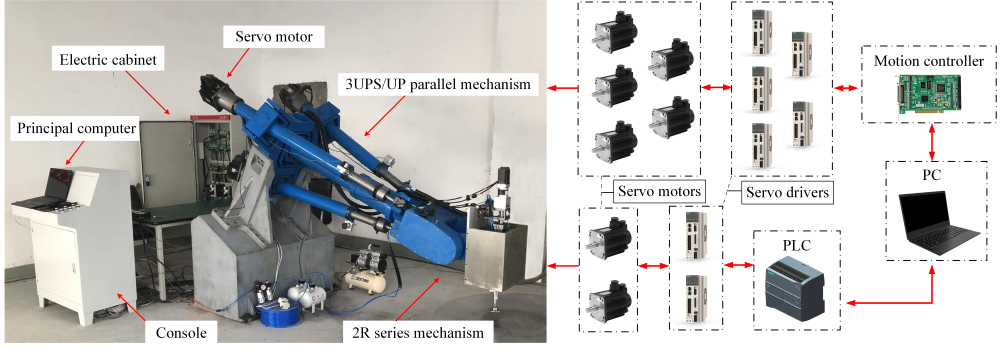
The 5-DOF hybrid mirror polishing robot is composed of three parts: the 3UPS/UP parallel mechanism, the 2R serial mechanism, and the dual-rotor grinding system. The prototype and its topological structure are shown in Fig. 1. In the process of optical mirror grinding and polishing, the dynamic characteristics and control accuracy of the parallel mechanism will largely affect the processing quality of the surface shape of the hybrid robot. Therefore, this paper mainly conducts dynamic modeling for the parallel mechanism and treats the effects of the 2R serial mechanism and the grinding system on the parallel mechanism as external loads.
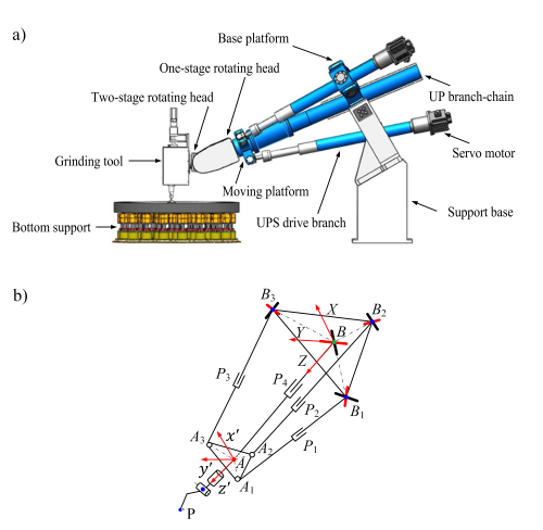
The 3UPS/UP parallel mechanism consists of a fixed platform B, a moving platform A, three UPS driving branched chains connecting the two, and one UP constraint branched chain. The three UPS branched chains AiBi (i = 1, 2, 3) are evenly distributed. Ball screws (P pairs) are installed in the branched chains. One end of each branched chain is connected to the moving platform A through a compound spherical hinge (S pair), and the other end is connected to the fixed platform B through a Hooke’s joint frame (U pair). A ball screw (P pair) is installed in the UP branched chain AB. This branched chain is arranged perpendicular to the moving platform A. One end is connected to the fixed platform B through a Hooke’s joint frame (U pair), and the other end is fixedly connected to the moving platform A. The 2R serial mechanism is composed of the first-stage rotor and the second-stage rotor. Among them, the first-stage rotor is connected to the moving platform through the turntable bearing, and the second-stage rotor is hinged to the first-stage rotor. The dual-rotor grinding system adopts the planetary motion mode, and the system consists of the revolution motor, the rotation motor, the pneumatic pressurizing device, the lapping and polishing disk, etc.
According to the right-hand rule, the connection points Bi (i=1,2,3) between the UPS branched chain and the fixed platform are the centers of Hooke’s hinges, and the connection points Ai (i=1,2,3) between the UPS branched chain and the moving platform are the centers of the compound spherical hinges. The connection points respectively form △B1B2B3 and △A1A2A3, both of which are equilateral triangles. Among them, point B is the geometric center of the fixed platform B1B2B3, and point A is the geometric center of the moving platform A1A2A3. In the fixed platform, a fixed coordinate system B-XYZ is established with B as the origin, where the X-axis coincides with the outer axis of the Hooke hinge of the UP branched chain, and the Z-axis is perpendicular to the plane of the fixed platform and points downward. To describe the motion of the UP branched chain and the moving platform relative to the fixed coordinate system, a moving platform attached coordinate system A-xyz is established on the moving platform with A as the origin, where the y-axis is parallel to the inner axis of the Hooke hinge of the UP branched chain, and the z-axis coincides with the motion axis of the UP branched chain. To describe the motion of the UPS branched chain at the end of the fixed platform, a driving branch chain attached coordinate system Bi-uiviwi is established at point Bi, where the vi-axis coincides with the inner axis of the Hooke hinge of the UPS branched chain, and the wi-axis coincides with the motion axis of the UPS branched chain. Additionally, a driving branch chain attached coordinate system Ai-uiviwi is established at point Ai, and the axes of this coordinate system are respectively parallel to those of the coordinate system Bi-uiviwi.
In the B-XYZ system, the closed-loop vector equation for the construction motion branch chain is constructed. The position and velocity vectors of point A can be expressed as:
{{\mathbf{r}}_A} = {{\mathbf{b}}_i} + {l_i} \cdot {{\mathbf{e}}_i} – {{\mathbf{a}}_i} = {l_j} \cdot {{\mathbf{e}}_j} \hfill \\
{{{\mathbf{\dot r}}}_A} = {{\text{v}}_i}{{\mathbf{e}}_i} + {l_i}{\omega _i} \times {{\mathbf{e}}_i} – {\omega _j} \times {{\mathbf{a}}_i} \hfill \\
{\text{ }} = {{\text{v}}_j}{{\mathbf{e}}_j} + {l_j}{\omega _j} \times {{\mathbf{e}}_j} \hfill \\
\end{gathered} \right.{\text{ }}\left( {i = 1,2,3,j = 4} \right).\quad \quad (1)$$
Among them, li and ei respectively represent the rod length and unit vector of the UPS driving branched chain, lj and ej respectively represent the rod length and unit vector of the UP constraint branched chain. Vectors bi and ai are respectively the position vectors of points Bi and Ai in the system B-XYZ; vi and vj respectively represent the axial linear velocity magnitudes of the UPS- and UP-branched chains; ωi and ωj respectively represent the angular velocity magnitudes of the UPS- and UP-branched chains. i and j respectively represent the UPS- and UP-branched chains. Furthermore, in the subsequent formulas of this article, the indices i and j are used in accordance with their definitions in Eq. (1).
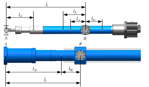
The distance from the centroid of the UPS branched chain located at the rear end of the fixed platform to the fixed hinge point Bi is lbi, and the distance from the centroid located at the front end of the fixed platform to the fixed hinge point Bi is lfi. The effective length of the UPS branched chain is li, and the distance from its centroid to the fixed hinge point Bi is lci. The distance from the rear end of the telescopic rod of the UPS branched chain to the moving hinge point Ai is lei. The UP branched chain is such that the distance from point A on the moving platform to point B on the fixed platform is lj, the distance from its center of mass to the fixed-point A on the moving platform is lAj, and the distance to the center point B on the fixed platform is lBj. The structural parameters of each branched chain are shown in Fig. 2.
According to the kinematic analysis, the velocities and accelerations of the centroids of each branch chain can be expressed as:
{{{\mathbf{\dot r}}}_{upsi}} = {{\mathbf{J}}_{ups}}{{{\mathbf{\dot r}}}_A}{\text{,}}\quad {{{\mathbf{\ddot r}}}_{upsi}} = {{\mathbf{J}}_{ups}}{{{\mathbf{\ddot r}}}_A} + {{{\mathbf{\dot J}}}_{ups}}{{{\mathbf{\dot r}}}_A}{\text{ }} \hfill \\
{{{\mathbf{\dot r}}}_{up}} = {{\mathbf{J}}_{up}}{{{\mathbf{\dot r}}}_A}{\text{,}}\quad \;\;{{{\mathbf{\ddot r}}}_{up}} = {{\mathbf{J}}_{up}}{{{\mathbf{\ddot r}}}_A} + {{{\mathbf{\dot J}}}_{up}}{{{\mathbf{\dot r}}}_A} \hfill \\
{{\mathbf{J}}_{ups}}{\text{ = }} – {{\dot l}_{fi}}{{\mathbf{e}}_{i \times }}\left( {{{\mathbf{e}}_{i \times }} + \left( {{\mathbf{e}}_i^{\text{T}}{{\mathbf{a}}_i}{{\mathbf{E}}_3} – {{\mathbf{a}}_i}{\mathbf{e}}_i^{\text{T}}} \right)\frac{{{{\mathbf{e}}_{j \times }}}}{{{l_j}}}} \right) \hfill \\
{{\mathbf{J}}_{up}} = {{\mathbf{e}}_j}{\mathbf{e}}_j^{\text{T}} – \left( {1 – \frac{{{l_{Aj}}}}{{{l_j}}}} \right)\left( {{{\mathbf{E}}_3} – {{\mathbf{e}}_j}{\mathbf{e}}_j^{\text{T}}} \right) \hfill \\
\end{gathered} \right..\quad \quad (2)$$
Among them, \( \mathbf{J}_{ups}, \mathbf{J}_{up}, \dot{\mathbf{J}}_{ups}, \dot{\mathbf{J}}_{up} \) respectively represent the Jacobian matrices and their derivatives. Specifically, they respectively represent the mapping relationship of the velocity and acceleration between the center point A of the moving platform and the UPS- and UP-branched chains. E3 is the third-order unit matrix, ei× and ej× respectively represent the third-order antisymmetric matrix of ei and ej, ejT is the transpose matrix of ej.
2.2 Joint Friction Model
The parallel mechanism has many joints and a complex structure. The contact between the joint motion pairs will produce variable friction phenomena. To facilitate the establishment of the friction force model, in this paper, only the joints of the UPS driving branch chain are modeled for friction, and the remaining joints are regarded as ideal motion pairs. In engineering practice, the “Coulomb + viscous” model is often used to express the friction effect. The connection joints of the three UPS branch chains with the moving platform and the static platform are respectively the composite spherical hinge and the Hooke’s hinge, and the corresponding friction force components are expressed as:
{f_{si}}(v) = {f_{vsi}}v + {f_{csi}}{\text{sgn}}(v) \hfill \\
{f_{hi}}(v) = {f_{vhi}}v + {f_{chi}}{\text{sgn}}(v) \hfill \\
\end{gathered} \right..\quad \quad (3)$$
In Eq. (3), fvhi, fvsi, fchi, and fcsi are respectively the viscous friction coefficients and the Coulomb friction coefficients at the Hooke’s joint and the compound spherical joint of the ith driving branched chain in the parallel mechanism, and v is the relative sliding speed of the contact surface, and sgn(·) denotes the sign function (if v < 0, sgn(v)= – 1, if v = 0, sgn(v)= 0 and if v > 0, sgn(v) = 1).
The compound spherical hinge connects the moving platform and the driving branched chain, and its joint reaction force is denoted as Fia. The Hooke’s hinge connects the fixed platform and the driving branched chain, and its joint reaction force is denoted as Fib. The friction torque components of the compound spherical hinge and the Hooke’s hinge in the driving branched chain are expressed as:
\left\{ \begin{gathered}
M_u^{asi} = \left[ {{f_{\nu si}}\omega _u^{ai}{R^{aui}} + {f_{csi}}\left\| {{\text{F}}_i^a} \right\|\operatorname{sgn} (\omega _u^{ai})} \right]{R^{aui}} \hfill \\
M_\nu ^{asi} = \left[ {{f_{\nu si}}\omega _\nu ^{ai}{R^{a\nu i}} + {f_{csi}}\left\| {{\text{F}}_i^a} \right\|\operatorname{sgn} (\omega _\nu ^{ai})} \right]{R^{a\nu i}} \hfill \\
M_w^{asi} = \left[ {{f_{\nu si}}\omega _w^{ai}{R^{awi}} + {f_{csi}}\left\| {{\text{F}}_i^a} \right\|\operatorname{sgn} (\omega _w^{ai})} \right]{R^{awi}} \hfill \\
\end{gathered} \right., \hfill \\
\left\{ \begin{gathered}
M_u^{bhi} = \left[ {{f_{\nu hi}}\omega _u^{bi}{R^{bui}} + {f_{chi}}\left\| {{\text{F}}_i^b} \right\|\operatorname{sgn} (\omega _u^{bi})} \right]{R^{bui}} \hfill \\
M_\nu ^{bhi} = \left[ {{f_{\nu hi}}\omega _\nu ^{bi}{R^{bvi}} + {f_{chi}}\left\| {{\text{F}}_i^b} \right\|\operatorname{sgn} (\omega _\nu ^{bi})} \right]{R^{bvi}} \hfill \\
\end{gathered} \right..\quad \quad (4) \hfill \\
\end{gathered}$$
In Eq. (4), ωuai, ωvai, and ωwai are respectively the rotational angular velocities of the composite spherical hinge around axes ui, vi, and wi. ωubi and ωvbi are respectively the rotational angular velocities of the Hooke’s joint about axes ui and vi. Raui, Ravi, and Rawi are the friction circle radii of the composite spherical hinge rotating joint, and Rbui and Rbvi are the friction circle radii of the Hooke’s hinge bearing.
2.3 The Normalized Dynamic Model Considering Joint Friction
2.3.1 Dynamic Analysis of Each Component
The UPS branched chain is subjected to Hooke’s hinge joint force Fib generated by the driving motor, the friction driving torque Mbhi, the reaction force Fia of the compound spherical hinge joint, the friction constraint torque Masi, and its own weight md g. The dynamic equilibrium equation of the driving branched chain is shown in Eq. (5).
{\mathbf{F}}_i^{\text{b}} – {\mathbf{F}}_i^{\text{a}} + {m_d}{\mathbf{g}} – {m_d}{{{\mathbf{\ddot r}}}_{upsi}} = 0 \hfill \\
{l_{ci}}\left( {{{\mathbf{e}}_i} \times {\mathbf{F}}_i^{\text{b}}} \right) – {l_i}\left( {{{\mathbf{e}}_i} \times {\mathbf{F}}_i^{\text{a}}} \right) + {l_{ci}}({{\mathbf{e}}_i} \times {m_d}{\mathbf{g}}) \hfill \\
\quad + {\mathbf{M}}_i^{{\text{bhi}}} – {{\mathbf{M}}^{asi}} + {{\mathbf{I}}_i}{{\dot \omega }_i} + {\omega _i} \times {{\mathbf{I}}_i}{\omega _i} = 0 \hfill \\
\end{gathered} \right.\quad . \quad \quad (5)$$
In Eq. (5), Ii = Ri Idi RiT, Idi is the moment of inertia of the driving branched chain in the coordinate system Bi – uiviwi.
The UP branched chain is subjected to the force and moment Fa and Ma from the moving platform, the reaction force and moment Fhb and Mhb from the Hooke’s hinge joint, and its own weight mcg. The dynamic equation of the constrained branched chain is shown in Eq. (6).
{{\mathbf{F}}^a} – {{\mathbf{F}}^{{\text{hb}}}} + {m_c}{\mathbf{g}} – {m_c}{{{\mathbf{\ddot r}}}_{up}} = 0 \hfill \\
{{\mathbf{M}}^a} – {{\mathbf{M}}^{hb}} + {l_{Aj}}\left[ {{{\mathbf{e}}_j} \times \left( {{{\mathbf{F}}^a}} \right)} \right] – {l_{Bj}}({{\mathbf{e}}_j} \times {{\mathbf{F}}^{hb}}) – {{\mathbf{I}}_j}{{\dot \omega }_j} – {\omega _j} \times {{\mathbf{I}}_j}{\omega _j} = 0 \hfill \\
\end{gathered} \right.. \quad \quad (6)$$
In Eq. (6), Ij = Rj Icj RjT, Icj is the moment of inertia of the driving branched chain in the coordinate system A-xyz.
The moving platform is subjected to the forces Fia from three compound spherical hinge joints, the frictional torque Masi, the reaction force and torque Fa and Ma from one UP branched chain, the reaction force and torque Fea and Mea from the equivalent external load, and its own weight mpg. The dynamic equilibrium equation of the moving platform is shown in Eq. (7).
In Eq. (7), Ip = Rp Idp RpT, Idp is the moment of inertia of the driving branched chain in the coordinate system A-xyz.
\mathop \sum \limits_{i = 1}^3 {\mathbf{F}}_i^a + {m_p}{\mathbf{g}} – {{\mathbf{F}}^a} – {\mathbf{F}}_e^a – {m_p}{{{\mathbf{\ddot r}}}_A} = 0 \hfill \\
\mathop \sum \limits_{i = 1}^3 {{\mathbf{M}}^{asi}} + \mathop \sum \limits_{i = 1}^3 {{\mathbf{a}}_i} \times {\mathbf{F}}_i^a – {{\mathbf{M}}^a} – {\mathbf{M}}_e^a – {{\mathbf{I}}_p}{{\dot \omega }_j} – {\omega _j} \times {{\mathbf{I}}_p}{\omega _j} = 0 \hfill \\
\end{gathered} \right..\quad \quad (7)$$
2.3.2 Parameter Normalization Dynamics Model
The dynamic model of the general form of the parallel mechanism can be expressed by Eqs. (5) to (7). However, this form of dynamic model cannot be used for the design of the dynamic controller. It is necessary to replace the kinematic parameters in the dynamic model with the kinematic parameters of the center point A of the moving platform and then construct the mapping model between the driving branch chain force and the pose of the center point of the moving platform.
The dynamic equation of the driving branched chain of the parallel mechanism is reconstructed as follows:
\begin{array}{*{20}{c}}
{{\mathbf{D}}_i^I{{{\mathbf{\ddot r}}}_A} + {\mathbf{D}}_i^C{{{\mathbf{\dot r}}}_A} + {\mathbf{D}}_i^f + {\mathbf{D}}_i^G = {{\mathbf{T}}_i}\quad \quad \quad \quad \quad \quad \quad \quad \quad \;\;\;\,} \\
{{\mathbf{D}}_i^I = {{\mathbf{e}}_{i \times }}{{\mathbf{I}}_i}{{\mathbf{J}}_{\omega i}} + {\mathbf{e}}_{i \times }^2{l_i}{m_d}{{\mathbf{J}}_i} – {\mathbf{e}}_{i \times }^2{l_i}{m_d}{{\mathbf{J}}_{upsi}}\quad \quad \quad \quad \quad \quad \;\;} \\
{{\mathbf{D}}_i^C = {{\mathbf{e}}_{i \times }}{{{\mathbf{\dot J}}}_{\omega i}} + {{\mathbf{e}}_{i \times }}{\left( {{{\mathbf{J}}_{\omega i}}{{{\mathbf{\dot r}}}_A}} \right)_{\times }}{{\mathbf{I}}_i}{{\mathbf{J}}_{\omega i}} – {\mathbf{e}}_{i \times }^2{l_i}{m_d}{{{\mathbf{\dot J}}}_i} – {{\mathbf{e}}_{i \times }}{l_i}{m_d}{{{\mathbf{\dot J}}}_{upsi}}} \\
{{\mathbf{D}}_i^f = {{\mathbf{e}}_{i \times }}{l_{ci}}{\mathbf{F}}_i^b – {{\mathbf{e}}_{i \times }}{l_i}{\mathbf{F}}_i^a + {{\mathbf{e}}_{i \times }}{\mathbf{M}}_i^{bhi} – {{\mathbf{e}}_{i \times }}{{\mathbf{M}}^{asi}}\quad \quad \quad \quad \quad \,} \\
{{\mathbf{D}}_i^G = \left( {{l_i} – {l_{ci}}} \right){m_d}{\mathbf{e}}_{i \times }^2{\mathbf{g}}\quad \quad \quad \quad \quad \quad \quad \quad \quad \quad \quad \quad \quad \;} \\
{{{\mathbf{J}}_{\omega i}} = \frac{1}{{{l_i}}}\left[ {{{\mathbf{e}}_{i \times }} + \left( {{\mathbf{e}}_i^{\operatorname{T}} {{\mathbf{a}}_i}{{\mathbf{E}}_3} – {{\mathbf{a}}_i}{\mathbf{e}}_i^{\operatorname{T}} } \right)\frac{{{{\mathbf{e}}_{j \times }}}}{{{l_j}}}} \right]\quad \quad \quad \quad \quad \quad \quad \quad } \\
{{{\mathbf{J}}_i} = {\mathbf{e}}_i^{\operatorname{T}} – \frac{{{\mathbf{e}}_i^{\operatorname{T}} {{\mathbf{e}}_j}{{\left( {{{\mathbf{a}}_i}} \right)}^{\operatorname{T}} }}}{{{l_j}}}\quad \quad \quad \quad \quad \quad \quad \quad \quad \quad \quad \quad \quad \quad }
\end{array}
\right..
\quad \quad (8)$$
The moving platform of the parallel mechanism is rigidly connected to the constraint branch chain, and its dynamic equation is reformulated as follows:
The normalized dynamic equation of the parallel mechanism is reformulated as shown in Eq. (10).
{\mathbf{D}}_4^I{{{\mathbf{\ddot r}}}_A} + {\mathbf{D}}_4^C{{{\mathbf{\dot r}}}_A} + {\mathbf{D}}_4^f + {\mathbf{D}}_4^G + {{\mathbf{D}}^E} = {{\mathbf{T}}_4} \hfill \\
{\mathbf{D}}_4^I = {{\mathbf{e}}_{j \times }}\left( {{{\mathbf{I}}_j} + {{\mathbf{I}}_p}} \right){{\mathbf{J}}_{\omega j}} + {\mathbf{e}}_{j \times }^2{l_{Bj}}{m_c}{{\mathbf{J}}_{\omega j}} + {\mathbf{e}}_{j \times }^2{l_{Bj}}{m_p}{{\mathbf{J}}_{up}} \hfill \\
{\mathbf{D}}_4^C = {{\mathbf{e}}_{j \times }}\left( {{{\mathbf{I}}_j} + {{\mathbf{I}}_p}} \right){{{\mathbf{\dot J}}}_{\omega j}} + {{\mathbf{e}}_{j \times }}{\left( {{{\mathbf{J}}_{\omega j}}{{{\mathbf{\dot r}}}_A}} \right)_ \times }\left( {{{\mathbf{I}}_j} + {{\mathbf{I}}_p}} \right){{\mathbf{J}}_{\omega j}} + {\mathbf{e}}_{j \times }^2{l_{Bj}}{m_c}{{{\mathbf{\dot J}}}_{up}} \hfill \\
{\mathbf{D}}_4^f = – {{\mathbf{e}}_{j \times }}{{\mathbf{M}}^{hb}} – {l_j}{\mathbf{e}}_{j \times }^2{{\mathbf{F}}^{hb}}{\text{ }} \hfill \\
{\mathbf{D}}_4^G = – {l_j}{m_c}{\mathbf{e}}_{j \times }^2{\mathbf{g}} – {l_{Bj}}{m_p}{\mathbf{e}}_{j \times }^2{\mathbf{g}} \hfill \\
{{\mathbf{D}}^E} = – {l_j}{\mathbf{e}}_{j \times }^2{\mathbf{F}}_e^a – {{\mathbf{e}}_{j \times }}{\mathbf{M}}_e^a \hfill \\
{{\mathbf{J}}_{\omega j}} = \frac{{{{\mathbf{e}}_{j \times }}}}{{{l_j}}} \hfill \\
\end{gathered} \right..\quad \quad (9)$$
In the formula, DI is the inertia matrix, DC is the coefficient matrix of centripetal and Coriolis forces, Df is the joint friction matrix, DG is the gravity matrix, DE is the external force matrix, and T = [t1 t2 t3] is the force matrix of the driving branched chain.
{\text{ }}{{\mathbf{D}}^I}{{\ddot r}_A} + {{\mathbf{D}}^C}{{\dot r}_A} + {{\mathbf{D}}^f} + {{\mathbf{D}}^G} + {{\mathbf{D}}^E} = {\mathbf{T}}, \hfill \\
\left\{ \begin{gathered}
{{\mathbf{D}}^I} = \mathop \sum \limits_{i = 1}^3 {\mathbf{D}}_i^I + {\mathbf{D}}_4^I{\text{ }},{\text{ }}{{\mathbf{D}}^C} = \mathop \sum \limits_{i = 1}^3 {\mathbf{D}}_i^C + {\mathbf{D}}_4^C \hfill \\
{{\mathbf{D}}^f} = \mathop \sum \limits_{i = 1}^3 {\mathbf{D}}_i^f + {\mathbf{D}}_4^f,{{\mathbf{D}}^G} = \mathop \sum \limits_{i = 1}^3 {\mathbf{D}}_i^G + {\mathbf{D}}_4^G \hfill \\
\end{gathered} \right..\quad \quad (10) \hfill \\
\end{gathered}$$
3 ERROR COMPENSATION ANALYSIS
3.1 The Influence of the Inertia on the Driving Force Error
The complete dynamic model of the parallel mechanism was established through derivation. However, this model is a complex nonlinear system, and there are problems such as large computational volume and poor real-time performance when it is directly used for motion control. Considering the low-speed characteristic in the optical mirror polishing process, in order to be more in line with the actual processing environment, the influence of the inertia parameters of each component on the driving force error was analyzed.
Based on the three-dimensional model of the polishing robot, parameter settings were carried out, and virtual prototype simulation tests were conducted. In order to facilitate the study of the variation law of the driving forces of each driving branched chain, based on the concentric circle trajectory of the actual optical processing, it was set that the center point A of the moving platform moved in a circular motion in the XY plane of the fixed coordinate system. The radius of the trajectory circle was 200 mm, and the running time for the center point of the moving platform was 1000 s. The trajectory equation is shown in Eq. (11).
X = 200\cos (0.002\pi t) \hfill \\
Y = 200\sin (0.002\pi t) \hfill \\
Z = 1300 \hfill \\
\end{gathered} \right..\quad \quad (11)$$
As shown in Fig. 3, in the low-speed motion state, when the inertia parameters of the UPS-driving branch chain, the UP-constraint branch chain, and the moving platform are ignored respectively, the output driving force error curves vary sinusoidally. The average maximum driving force errors of the three driving branch chains are 15.3 N, 52.1 N, and 34.5 N, respectively. It can be seen that the inertia parameter of the UPS-driving branch chain has the least influence on the driving force output by the model and can thus be neglected to simplify the dynamic model. Through model simplification, the calculation time can be reduced. However, since the inertia of the driving branch chain is directly ignored, a certain driving force error will be generated, thereby affecting the motion control accuracy of the mechanism. Therefore, the output driving force error needs to be compensated.
3.2 Driving Force Error Compensation Mode
Elman neural network has excellent dynamic memory and time-varying characteristics, enabling it to handle relatively complex information and making it highly suitable for the online compensation of the error in the simplified dynamic model of the parallel mechanism of the polishing robot. However, the traditional Elman neural network randomly initializes the weight and threshold matrices. Its prediction accuracy is easily influenced by these parameters, leading to a slow network learning speed and low prediction accuracy. Therefore, it is necessary to optimize the weights and thresholds of the neural network. The WOA has been applied more due to its fewer parameters and simpler structure. In this paper, based on this algorithm, the parameters of the neural network are optimized, then an error compensation model is built. The process of the whale algorithm is shown in the following Table 1.
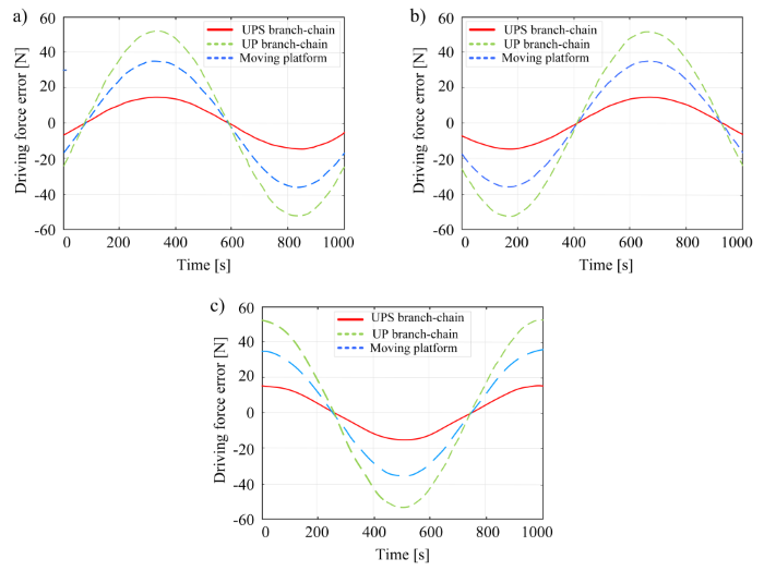
Table 1. Algorithm flow of WOA
| Algorithm. Search for the optimal whale individual |
|---|
|
Input: the population size to N 2: Check if any whale individual exceeds the search space 5: While t < tmax |
To enable a more intuitive comparison of the driving force error compensation performance between Elman and WOA-Elman neural network, the prediction accuracy of both models is evaluated using three quantitative metrics: mean absolute error (MAE), mean absolute percentage error (MAPE), and root mean square error (RMSE). Among these metrics, the values of MAE, MAPE, and RMSE are inversely related to the prediction accuracy of the neural network model: higher values indicate lower predictive accuracy. The mathematical expressions for MAE, MAPE, and RMSE are as follows:
{\text{MAE}} = \frac{1}{n}\mathop \sum \limits_{i = 1}^n \left| {{{\hat \tau }_i} – {\tau _i}} \right| \hfill \\
{\text{MAPE}} = \frac{1}{n}\mathop \sum \limits_{i = 1}^n \left| {\frac{{{{\hat \tau }_i} – {\tau _i}}}{{{\tau _i}}}} \right| \hfill \\
{\text{RMSE}} = \sqrt {\frac{1}{n}\mathop \sum \limits_{i = 1}^n {{\left( {{{\hat \tau }_i} – {\tau _i}} \right)}^2}} \hfill \\
\end{gathered} \right..\quad \quad (12)$$
In the equations, \( \widehat{\tau}_i \) and τi denote the driving force values generated by the simplified dynamic model and the complete dynamic model at the ith time step, respectively.
The center point of the moving platform follows the trajectory defined by Eq. (11). The position, velocity, and acceleration vectors of this point are obtained through numerical simulation and serve as input samples for the neural network. The corresponding driving force data are then computed using both simplified and complete dynamic models. Subsequently, the evaluation metrics for driving force error prediction were computed for both the Elman and WOA-Elman models, with the results presented in Table 2.
Table 2. Evaluation metrics for driving force prediction
| Neural network | Maximum error [N] | MAE [N] | MAPE [%] | RMSE [N] |
|---|---|---|---|---|
| Elman | 0.139 | 0.047 | 1.273 | 0.041 |
| WOA-Elman | 0.007 | 0.003 | 0.146 | 0.002 |
As shown in Table 2, WOA-Elman neural network achieves a relatively low prediction error, thereby significantly enhancing driving force prediction accuracy, with a maximum error of only 0.007 N. It effectively compensates for driving force errors arising from dynamic model simplification.
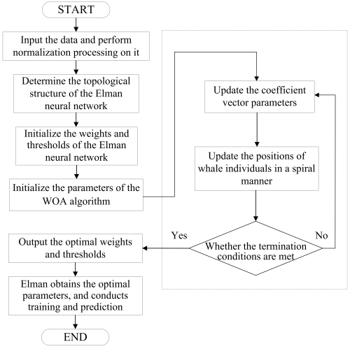
The WOA is first adopted to optimize the weights and thresholds between the layers of Elman neural network. Then, the optimized Elman neural network using WOA is used to construct a dynamic error compensation model, achieving accurate prediction and real-time compensation for the driving force error, and ensuring the accuracy of the dynamic model of the parallel mechanism to the maximum extent. The driving force error compensation process constructed by the WOA-Elman model is shown in Fig. 4.
It is known from the dynamic model of the parallel mechanism that the driving force of the UPS branched chain is related to the position and posture of the center point A of the moving platform. Therefore, vector Q, which is composed of the position of the center point of the moving platform of the parallel mechanism, its first derivative, and its second derivative, is taken as the input of the neural network, and the driving force error \( \Delta \mathbf{T} \) is taken as the output of the neural network.
\begin{gathered}
{\mathbf{Q}} = {({{\mathbf{r}}_A},{{{\mathbf{\dot r}}}_A},{{{\mathbf{\ddot r}}}_A})^{\operatorname{T}} } = {[x,y,z,\dot x,\dot y,\dot z,\ddot x,\ddot y,\ddot z]^{\operatorname{T}} } \hfill \\
\Delta {\mathbf{T}} = {\left[ {\vartriangle {t_1},\vartriangle {t_2},\vartriangle {t_3}} \right]^{\operatorname{T}} } \hfill \\
\end{gathered}
\right..
\quad \quad (13)$$
The dynamic model of the polishing robot can be reconstructed by compensating for the driving force error through WOA-Elman neural network as follows:
4 SLIDING MODE CONTROL ALGORITHM
4.1 The Analysis and Design of the Reaching Law
The process in which the system approaches the switching surface from any initial state is called the reaching motion. The common reaching laws that describe the reaching motion include the constant velocity reaching law, the exponential reaching law, and the power reaching law, etc. The exponential reaching law (Eq. (15)) has a faster reaching speed when it is far from the sliding mode surface, enabling the system to reach the vicinity of the switching surface faster. However, due to the use of the sign function in the switching term, it causes large chattering in the system when it is close to the sliding mode surface. In this paper, based on the power reaching law (Eq. (16)), an improved reaching law is designed by adding a variable-speed reaching term K.
Among them, ε, k, k1, k2, k3, \( \sigma \), and \( \alpha \) are all parameters of the reaching law, and all these parameters are greater than zero, with \( \alpha \) > 1. In the variable-speed reaching term, er represents the trajectory tracking error.
In the variable speed approaching term K, when the distance from the sliding mode surface is large, the trajectory tracking error is large. The variable speed term tends to the constant k3, and the influence of the variable speed term on the approaching process is small. At this time, the power term plays a major role, enabling the system to converge rapidly to the vicinity of the sliding mode surface. When the distance from the sliding mode surface is small, the power term approaches zero. At this time, the variable speed term plays a major role, and the value of the variable speed term decreases as the system variable decreases, allowing the system to approach the sliding mode surface more smoothly. However, the switching function in the variable-speed term is defined as the sign function sgn(s). Due to its inherent switching characteristics, this introduces chattering into the system. To mitigate this issue, the smooth hyperbolic tangent function tanh(s) is employed as a substitute for the sign function, thereby reducing the chattering effect. Consequently, the improved reaching law is presented in Eq. (18).
\dot s = – {k_1}{\left| s \right|^\alpha }\operatorname{sgn} (s) – {k_2}s – {k_3}\frac{{\left| {{e_r}} \right|}}{{\left| {{e_r}} \right| + \sigma }}{\text{tanh}}(s) \hfill \\
s = c{e_r} + {{\dot e}_r},\quad c > 0 \hfill \\
\tanh (s) = \frac{{{{\text{e}}^s} – {{\text{e}}^{ – s}}}}{{{{\text{e}}^s} + {{\text{e}}^{ – s}}}} \hfill \\
\end{gathered} \right..\quad \quad (18)$$
4.2 The Design of a Nonlinear Disturbance Observer
In the control system, factors such as external interference or unmodeled errors can affect control accuracy. The disturbance observer estimates the effects of these uncertain factors and introduces an error compensation term at the input end of the controller to ultimately eliminate the impact of these errors on control accuracy.
Introducing the external disturbance d, the dynamic model of the parallel mechanism control system is organized as follows:
It is defined that \( \widehat{\mathbf{d}} \) is the estimate of the external disturbance d, εd is the disturbance observation error, and z is the auxiliary parameter vector. It can be seen from this that:
{{\mathbf{\varepsilon }}_d} = {\mathbf{d}} – \widehat {\mathbf{d}} \hfill \\
{\mathbf{z}} = \widehat {\mathbf{d}} – {\mathbf{p}}\left( {{{\mathbf{r}}_A},{{{\mathbf{\dot r}}}_A}} \right) \hfill \\
\begin{array}{*{20}{c}}
{\widehat {{\mathbf{\dot d}}}}
\end{array} = {\mathbf{L}}\left( {{{\mathbf{r}}_A},{{{\mathbf{\dot r}}}_A}} \right){{\mathbf{\varepsilon }}_d} \hfill \\
\end{gathered} \right.,\quad \quad (20)$$
Among them, there are the following variables: P denotes the function vector, and L represents the gain matrix of the disturbance observer. These are required to satisfy Eq. (21).
{\frac{{\partial {\mathbf{p}}\left( {{{\mathbf{r}}_A},{{{\mathbf{\dot r}}}_A}} \right)}}{{\partial {{\mathbf{r}}_A}}}}&{\frac{{\partial {\mathbf{p}}\left( {{{\mathbf{r}}_A},{{{\mathbf{\dot r}}}_A}} \right)}}{{\partial {{{\mathbf{\dot r}}}_A}}}}
\end{array}} \right]\left[ {\begin{array}{*{20}{c}}
{{{{\mathbf{\dot r}}}_A}} \\
{{{{\mathbf{\ddot r}}}_A}}
\end{array}} \right].\quad \quad (21)$$
The first-order derivative of z can be obtained as shown in Eq. (22).
{\widehat {{\mathbf{\dot d}}}}
\end{array} – \frac{{d{\mathbf{p}}({{\mathbf{r}}_A},{{{\mathbf{\dot r}}}_A})}}{{dt}} = \begin{array}{*{20}{c}}
{\widehat {{\mathbf{\dot d}}}}
\end{array} – {\mathbf{L}}\left( {{{\mathbf{r}}_A},{{{\mathbf{\dot r}}}_A}} \right){{\mathbf{D}}^I}{{\mathbf{\ddot r}}_A}.\quad \quad (22)$$
The nonlinear disturbance observer is designed as follows:
{\mathbf{\dot z}} = {\mathbf{L}}\left( {{{\mathbf{r}}_A},{{{\mathbf{\dot r}}}_A}} \right)\left( \begin{gathered}
{{\mathbf{D}}^C}{{{\mathbf{\dot r}}}_A} + {{\mathbf{D}}^f} + {{\mathbf{D}}^G} \hfill \\
+ {{\mathbf{D}}^E} + \Delta {\mathbf{T}} – {\mathbf{T}} \hfill \\
– {\mathbf{p}}\left( {{{\mathbf{r}}_A},{{{\mathbf{\dot r}}}_A}} \right) \hfill \\
\end{gathered} \right) – {\mathbf{L}}\left( {{{\mathbf{r}}_A},{{{\mathbf{\dot r}}}_A}} \right){\mathbf{z}} \hfill \\
\widehat {\mathbf{d}} = {\mathbf{z}} + {\mathbf{P}}\left( {{{\mathbf{r}}_A},{{{\mathbf{\dot r}}}_A}} \right) \hfill \\
\end{gathered} \right..\quad \quad (23)$$
4.3 Trajectory Tracking Controller Design
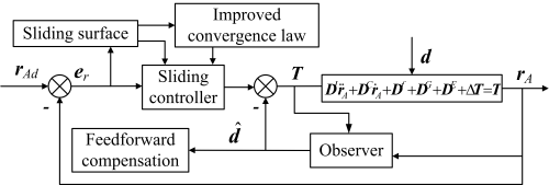
When designing the trajectory tracking controller for the parallel mechanism of the polishing robot, by combining the analysis of the improved reaching law and the nonlinear disturbance observer, the control law u is designed to continuously adjust the motion state based on the real-time feedback pose rA of the center point of the moving platform, ensuring that the parallel mechanism accurately tracks the expected pose rAd of the center point of the moving platform. The structure design of the sliding mode controller is shown in Fig. 5.
The trajectory tracking controller is designed as shown in Eq. (24).
{\mathbf{u}} = {{\mathbf{D}}^I}\left( {{{{\mathbf{\ddot r}}}_{Ad}} + {\mathbf{c}}{{{\mathbf{\dot e}}}_r}} \right) + {{\mathbf{D}}^C}\left( {{{{\mathbf{\dot r}}}_{Ad}} + {\mathbf{c}}{{\mathbf{e}}_r}} \right) + {{\mathbf{D}}^f} + {{\mathbf{D}}^G} + {{\mathbf{D}}^E} \\
+ \Delta {\mathbf{T}} – \widehat {\mathbf{d}} + {{\mathbf{K}}_1}{\left| {\mathbf{s}} \right|^\alpha }\operatorname{sgn} ({\mathbf{s}}) + {{\mathbf{K}}_2}{\mathbf{s}} + {{\mathbf{K}}_3}\frac{{\left| {{{\mathbf{e}}_r}} \right|}}{{\left| {{{\mathbf{e}}_r}} \right| + \sigma }}\tanh ({\mathbf{s}}) \\
{\mathbf{s}} = {\mathbf{c}}{{\mathbf{e}}_r} + {{{\mathbf{\dot e}}}_r} \\
\end{gathered} \right..\quad \quad (24)$$
Among them, u is the sliding mode control law, and s is the sliding surface.
5 EXPERIMENTS AND DISCUSSION
5.1 Simulation Analysis of Trajectory Tracking Control
5.1.1 Simulation Platform Construction and Parameter Selection
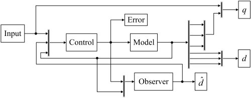
In order to verify the effects of the improvements in the reaching law and the design of the nonlinear disturbance observer, a simulation experiment was conducted on the trajectory tracking control system of the polishing robot parallel mechanism. The simulation structure of the control system is shown in Fig. 6, where “Input” represents the expected trajectory input for the parallel mechanism, “Control” refers to the sliding mode controller whose output is the driving force, “Model” denotes the dynamic model of the parallel mechanism whose output includes the actual trajectory and actual disturbance, and “Observer” indicates the nonlinear disturbance observer whose output is the disturbance estimation value.
The simulation trajectory of the center point of the moving platform is as shown in Eq. (11). The simulation duration is set to 100 s, and the initial position of the mechanism is (190 mm, 10 mm, 990 mm). The parameters related to the exponential reaching law and the improved reaching law are taken as ε = 10, k = 750, k1 = 20, k2 = 750, k3 = 20, α = 2, σ = 5. Meanwhile, external interference d(t)=[10sin(0.01t), 10sin(0.01t), 10sin(0.01t)]T is added during the simulation. The relevant parameters of the hybrid polishing robot are presented in Table 3.
Table 3. The relevant parameters of the hybrid polishing robot
| Parameters | Value | Parameters | Value | |
|---|---|---|---|---|
| md | 95 kg | Raui | 10 mm | |
| mc | 117 kg | Ravi | 8.5 mm | |
| mp | 32 kg | Rawi | 15 mm | |
| r | 150 mm | Rbui | 25 mm | |
| R | 400 mm | Rbvi | 25 mm | |
| lei | 657 mm | fvhi; fvsi | 0.02 | |
| lAj | 820 mm | fchi; fcsi | 0.05 |
5.1.2 Analysis of Simulation Results
In order to verify the effectiveness of the designed sliding mode control algorithm, three sets of simulation control experiments were established. The first set was used to verify the influence of the nonlinear disturbance observer on the dynamic characteristics and control accuracy of the traditional sliding mode control system based on the exponential reaching law. The second set was used to verify the influence of the improved reaching law on the convergence speed of the sliding mode control system based on the nonlinear disturbance observer. The third set was used to verify the suppression effect of different reaching laws on the chattering of the sliding mode control system based on the nonlinear disturbance observer. The simulation experiment results are shown in Figs. 7 and 8.
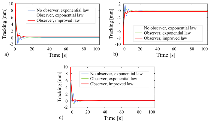
It can be seen from Fig. 7 that under the same exponential reaching law, the system adjustment times in the X, Y, and Z directions are relatively close, approximately 12.5 s. However, the nonlinear disturbance observer has different effects on error fluctuations. When there is no observer, the error fluctuations are relatively large. In all three directions, the mean value of the maximum fluctuating error amplitude is approximately 1.92 mm. When there is an observer, the error fluctuations are relatively small, and the mean value of the maximum fluctuating error amplitude is approximately 1.14 mm. The simulation results show that the designed nonlinear disturbance observer can effectively resist external disturbances, enabling the control system to have better dynamic characteristics and error compensation capabilities. This is because the control law switching gain of the traditional sliding mode control system based on the exponential reaching law is relatively low. Without the assistance of a disturbance observer, such a low control law switching gain cannot guarantee the required control accuracy.
Under the condition of having a nonlinear disturbance observer, the adjustment time of the improved reaching law system in the X, Y, and Z directions is approximately 9 s. The convergence speed is increased by approximately 28 % compared with that of the exponential reaching law. The mean value of the maximum fluctuation error amplitude is approximately 0.27 mm, and the control accuracy is further improved.
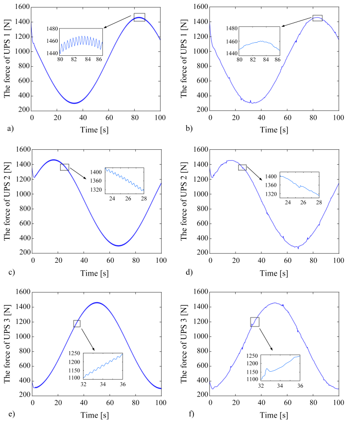
As demonstrated in Fig. 8, the sliding mode control system with a nonlinear disturbance observer, when employing the exponential reaching law, exhibits high-frequency chattering in the driving force output curve. This phenomenon can be attributed to the switching term of the exponential reaching law, which is a sign function. The inherent nature of the sign function dictates its chattering characteristics. Despite the nonlinear disturbance observer’s ability to effectively counteract external disturbances and permit the use of smaller switching gains, the control system still experiences high-frequency chattering. In contrast, the enhanced reaching law adopts a continuous and smooth hyperbolic tangent function as the switching term when approaching the sliding surface, which significantly suppresses system chattering.
5.2 Experimental Analysis of Trajectory Tracking Control
In order to verify the actual effect of the designed sliding mode control algorithm, an experimental platform is built as shown in Fig. 9. The experimental platform includes a optical mirror polishing robot, an upper computer, an electrical control cabinet, a servo control system, an integrated multi-axes controller motion control card, and corresponding sensors. The servo control system of the parallel mechanism, which respectively controls the three active branches. The servo control system of the series mechanism, which respectively controls the two-stage rotors. All five sets of servo systems are controlled by the IMAC motion control card. The dual-rotor grinding system includes two sets of servo drivers and servo motors and is controlled by the Siemens S7-1200 series PLC. In this experiment, the axial displacement data of the three active branches of the parallel mechanism are obtained through the linear displacement sensor and the encoder of the driving motor. The pose data of the center point of the moving platform is obtained through the forward kinematics solution.
5.2.1 Analysis of Experimental Results
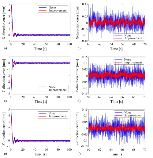
Based on the position of the polishing table, the initial position of the moving platform’s center point of the polishing robot was set to (195 mm, 5 mm, 995 mm), with a sampling time of 2 ms. The desired trajectory was selected as a simple circular trajectory, as shown in Eq. (11). Trajectory tracking experiments were conducted using both conventional sliding mode control and sliding mode control based on a nonlinear disturbance observer with an enhanced reaching law. To reduce the contingency of a single experiment, the average value of five control experiments was taken as the result. The trajectory tracking error curve and the locally enlarged error curve of the moving platform’s center point were plotted, as shown in Fig. 10.
As shown in Fig. 10, the enhanced sliding mode control algorithm demonstrates significant advantages over conventional sliding mode control in terms of trajectory tracking error fluctuations, convergence speed, and control precision. To provide a more intuitive comparison of the trajectory tracking control precision between the two algorithms, the tracking errors between 60 s and 70 s of the experimental process were magnified by a factor of 10. It can be observed that the trajectory tracking errors of the conventional sliding mode control in the X, Y, and Z directions of the moving platform’s center point fluctuate within the ranges of −0.122 mm to 0.147 mm, −0.124 mm to 0.130 mm, and −0.129 mm to 0.133 mm, respectively. In contrast, the enhanced sliding mode control algorithm significantly reduces the fluctuation amplitude of the trajectory tracking errors, with the fluctuation ranges reduced to −0.058 mm to 0.067 mm, −0.049 mm to 0.054 mm, and −0.056 mm to 0.065 mm, respectively.
6 CONCLUSIONS
This paper proposes a dynamics-based sliding mode control strategy to improve the working performance of a 5-DOF hybrid polishing robot. Firstly, kinematic analysis is carried out based on the closed vector method, and the dynamic model with joint friction effect is established by using the Newton-Euler method. Through the substitution of kinematic parameters, an explicit dynamic model between the driving force of the driving branched chain and the pose of the center point of the moving platform is constructed. Secondly, to balance the relationship between the model solution efficiency and control accuracy, the influence of the inertia parameters of each component of the parallel mechanism on the driving force is evaluated. The dynamic model is simplified, and the error term is corrected by using the WOA-Elman algorithm, reconstructing the dynamic model with an error compensation term. Finally, to improve the robustness and pose accuracy of the trajectory tracking control system, an end trajectory sliding mode control algorithm is proposed based on the analysis of the reaching law and the design of the nonlinear disturbance observer. Simulation and experimental results show that by adding the improved reaching term, the system chattering can be effectively reduced, and by using the nonlinear disturbance observer to estimate the system error and external disturbance, the error fluctuation and convergence speed of the system in the convergence process can be effectively reduced, verifying the robustness and high accuracy of the trajectory tracking control system of the polishing robot.
However, this study also has certain limitations. Increasing the gain of the control system enhances its anti-interference ability, reduces the trajectory tracking error, and leads to a better control effect. But when the system is close to the sliding mode surface, a smaller gain is required to weaken the chattering. Therefore, in future work, more in-depth research is needed on the adaptive adjustment algorithm of the control system gain.
References
- Li, S.S., Wang, H.B., Li, M.H., Li, L.Q., Yang, J., Niu, J.Y., et al. Kinematics and performance analysis of a parallel 4-UPS/RRR trunk rehabilitation robot. J Mech Sci Technol 38 6319-6333 (2024) DOI:10.1007/s12206-024-1043-7.
- Liang, X., Zeng, X., Li, G., Chen, W., Su, T., He, G. Design, analysis, and optimization of a kinematically redundant parallel robot. Actuators 12 120 (2023) DOI:10.3390/act12030120.
- Elsamanty, M., Faidallah, E.M., Hossameldin, Y.H., Rabbo, S.A., Maged, S.A., Yang, H.B., et al. Workspace Analysis and path planning of a novel robot configuration with a 9-DOF serial-parallel hybrid manipulator (SPHM). Appl Sci (Basel) 13 2088 (2023) DOI:10.3390/app13042088.
- Dong, K.F., Li, J., Lv, M.Y., Li, X., Gu, W., Cheng, G. Active disturbance rejection control algorithm for the driven branch chain of a polishing robot. Stroj vestn-J Mech Eng 69 509-521 (2023) DOI:10.5545/sv-jme.2023.680.
- Jallet, W., Bambade, A., Mansard, N., Carpentier, J. Constrained differential dynamic programming: A primal-dual augmented Lagrangian approach. IEEE Int Conf Intell Robot Syst 13371-13378 (2022) DOI:10.1109/IROS47612.2022.9981586.
- Zhang, C.X., Zhao, Y.Q., Shen, Y.W., Li, D.Y. The modeling and analysis of vibration response with airdrop vehicle in landing process. J Braz Soc Mech Sci Eng 46 345 (2024) DOI:10.1007/s40430-024-04913-y.
- Chen, Y.L., Sun, Q., Guo, Q., Gong, Y.J. Dynamic modeling and experimental validation of a water hydraulic soft manipulator based on an improved Newton-Euler iterative method. Micromachines (Basel) 13 130 (2022) DOI:10.3390/mi13010130.
- Raj, M.A.H., Nair, V.G. Dynamics analysis and simulation of a six degree of freedom wobbling platform using Lagrangian method. IEEE Access 12 172867-172878 (2024) DOI:10.1109/ACCESS.2024.3492202.
- Guo, F., Cheng, G., Pang, Y. Explicit dynamic modeling with joint friction and coupling analysis of a 5-DOF hybrid polishing robot. Mech Mach Theory 167 104509 (2022) DOI:10.1016/j.mechmachtheory.2021.104509.
- Hou, Y.L., Deng, Y.J., Zeng, D.X. Dynamic modelling and properties analysis of 3RSR parallel mechanism considering spherical joint clearance and wear. J Cent South Univ 28 712-727 (2021) DOI:1007/s11771-021-4640-y.
- Fischer, O., Toshimitsu, Y., Kazemipour, A., Katzschmann, R.K. Dynamic task space control enables soft manipulators to perform real-world tasks. Adv Intell Syst 5 2200024 (2023) DOI:10.1002/aisy.202200024.
- Yang, Z.Y., Sun, M.L., Li, W.Q., Liang, W.Y. Modified Elman network for thermal deformation compensation modeling in machine tools. Int J Adv Manuf Technol 54 669-676 (2011) DOI:10.1007/s00170-010-2961-3.
- Su, M.Y., Chen, Y.M., Li, Q., Wei, Y., Liu, J.S., Chang, Z.W., et al. Temperature compensation model for non-dispersive infrared CO gas sensor based on WOA-BP algorithm. Fron Energy Res 12 1407630 (2024) DOI:10.3389/fenrg.2024.1407630.
- Chen, F.J., Liao, J.Q., Xiong, J., Yin, S.H., Huang, S., Tang, Q.C. High-precision trajectory tracking design and simulation for six degree of freedom robot based on improved active disturbance rejection control. Proc Inst Mech Eng C-J Mech 233 3659-3669 (2019) DOI:10.1177/0954406218813397.
- Pak, Y.J., Kong, Y.S., Ri, J.S. Robust PID optimal tuning of a Delta parallel robot based on a hybrid optimization algorithm of particle swarm optimization and differential evolution. Robotica 41 1159-1178 (2023) DOI:10.1017/S0263574722001606.
- Li, X.H., Liu, X.P., Wang, G., Gu, K.Q., Che, H.L. Discrete open-closed-loop PID-type iterative learning control for trajectory tracking of tracked mobile robots. Int J Adv Robot Syst 19 (2022) DOI:10.1177/17298806221137247.
- Ahmed, T., Islam, M.R., Brahmi, B., Rahman, M.H. Robustness and tracking performance evaluation of PID motion control of 7 DoF anthropomorphic exoskeleton robot assisted upper limb rehabilitation. Sensors 22 3747 (2022) DOI:10.3390/s22103747.
- Yang, Q., Zhang, F., Wang, C. Deterministic learning-based neural PID control for nonlinear robotic systems. IEEE/CAA J Autom Sin 11 1227-1238 (2024) DOI:10.1109/JAS.2024.124224.
- Madebo, N.W., Abdissa, C.M., Lemma, L.N. Enhanced trajectory control of quadrotor UAV using fuzzy PID based recurrent neural network controller. IEEE Access 12 190454-190469 (2024) DOI:1109/ACCESS.2024.3516494.
- Saoudi, K., Bdirina, K., Guesmi, K. Robust estimation and control of uncertain affine nonlinear systems using predictive sliding mode control and sliding mode observer. Int J Syst Sci 55 1480-1492 (2024) DOI:10.1080/0020 7721.2024.23061913.
- Li, Z.Y., Zhai, J.Y. Super-twisting sliding mode trajectory tracking adaptive control of wheeled mobile robots with disturbance observer. Int J Robust Nonlinear Contr 32 9869-9881 (2022) DOI:10.1002/rnc.634.
- Shan, W.T., Zhao, J.Q., Han, Z.H. Novel dual-sliding mode sensorless vector control strategy for permanent magnet synchronous motorized spindles. J Mech Sci Technol 38 6895-6905 (2024) DOI:10.1007/s12206-024-1140-7.